In my economics education, most of the statistics and econometrics I had learnt focused on adopting an explanatory lens. We want to establish whether something has a significant effect on the outcome of interest, and we apply econometric techniques of varying complexity (typically some form of regression analysis e.g. instrument variables regression, diff-in-diff) to get around various biases (e.g. omitted variable bias, reverse causality) that would result in some form of biased estimate.

That form of data analysis is inherently quite backward looking - not totally, because the end-goal of that research is still to apply the lessons to the future (e.g. future policy). But I observe that the “data analysis” that is desirable in today’s world is a more forward-looking type of data analysis, where we take lessons from existing data to explicitly model or predict future data. Hence, the lens is more of a predictive lens rather than explanatory lens.

The two are not quite the same. Understanding the causal factors and the causal effect will naturally contribute to good prediction. But what if you have a precisely estimated effect for a factor that, in the bigger scheme of things, is just a small driver of the overall outcome of interest? Conversely, what if I could predict the outcome reliably using an observable, without knowing the causal mechanism that links the two?

These days, the buzzword in such predictive data analysis is probably machine learning. It sounds daunting, though in reality there is a natural bridge from what I have learnt in the past to the machine learning world; as it turns out, regression is both an econometric technique and a machine learning technique too.

That brings me to tidymodels. I had started learning R using the tidyverse packages and more recently I started learning about the tidymodels package. I guess I think of it as a companion package to tidyverse that focuses on modelling and machine learning - seems to fit in seamlessly with the tidyverse as a whole.

The basics are not that hard to get into, and I will illustrate using the coffee ratings data from TidyTuesday.

Basic use of tidymodels

After loading and inspecting the data (see instructions in the link above for how to get the data), the first thing I do is a bit of pre-cleaning the data. I want to focus on Arabica beans so I remove the minority of Robusta entries. I also want to remove data for which the combination of country of origin and coffee bean variety has too few data points, as the model will not be trained well if there are too few data points within that category. This process cost me 15.8% of the total observations.

Note: Most of the variables I use to model are categorical variables, hence there is additional complexity with having not enough variability within/across combinations of categories. If most predictors are numerical (i.e. continuous), this would be less of an issue.

At this stage, there is no need to do serious data manipulation/wrangling, as these will be covered by the data prep steps later.

coffee_ratings_filtered <- coffee_ratings %>%
  filter(species == "Arabica") %>%  
  ## remove small number of Robusta entries (only interested in Arabica)
  
  group_by(country_of_origin, variety) %>%   
  filter(n() >= 5)
  ## filter out countries/variety combinations with too few data points as the training will not be good
  ## on the other hand, can't set too strict a filter or we lose too many data points overall

coffee_ratings_filtered %>% group_by(country_of_origin, variety) %>% 
  summarise(n())

glimpse(coffee_ratings_filtered)

Next, we divide the data into training and test data (75-25 split in this case). The model will be trained on the training data, and will not use the test data. The test data is set aside as “new data” to test our model.

set.seed(42) #for replicability

coffee_split <- initial_split(coffee_ratings_filtered, 
                              prop = 0.75, #use 75% for training set
                              strata = total_cup_points)

coffee_training <- coffee_split %>% training()
coffee_test <- coffee_split %>% testing()

After that, we define how we want to prep the data (“recipe”) then apply the steps to the data (“prep”/”bake”). The tidymodels package has these helpful recipe steps, so I don’t have to do all these data cleaning and preparation manually.

In this case, I have specified that I want to regress the coffee ratings on country of origin, the coffee varietal, the processing method, the altitude, and the number of category one and two defects. In practice, the model will be trained iteratively to figure out which are the best predictors to use.

coffee_recipe <- recipe(total_cup_points ~ country_of_origin + variety + processing_method + altitude_mean_meters + category_one_defects + category_two_defects,
                        data = coffee_training) %>%
  step_normalize(altitude_mean_meters) %>% ## normalise numerical predictors
  step_string2factor(all_nominal_predictors()) %>% ## convert characters to factors
  step_novel(all_nominal_predictors()) %>% ## handles new levels in the test set not seen in the training set
  step_dummy(all_nominal_predictors()) ## encode factors into dummies

coffee_training_prep <- coffee_recipe %>%
                      prep(training = coffee_training) %>%
                      bake(new_data = NULL)
                      # prep the training data using the recipe

coffee_test_prep <- coffee_recipe %>%
                    prep(training = coffee_training) %>%
                    bake(new_data = coffee_test)
                    # prep the test data using the recipe

Having prepped the training (and test) data, we can now train the model. I define the model that I want to use, i.e. linear regression, and then apply that model to fit the prepped training data.

lm_model <- linear_reg() %>%
            set_engine('lm') %>%
            set_mode('regression') #define the model. here i use linear regression

lm_fit <- lm_model %>%
          fit(total_cup_points ~ .,
              data = coffee_training_prep)

With the trained model, we now apply it to the test data (i.e. “new data”) to produce the predicted value of the outcome variable (i.e. coffee ratings).

coffee_predictions <- lm_fit %>% 
                      predict(new_data = coffee_test_prep)

coffee_test_results <- coffee_test %>%
                      bind_cols(coffee_predictions)

Because we know the true value of the coffee ratings from the data set, we can compare the predicted value to the true value to assess our model. Root mean squared error (RMSE) and r-squared are two common metrics to assess model performance.

coffee_test_results %>% 
  group_by(country_of_origin) %>%
  rmse(truth = total_cup_points, estimate = .pred)

coffee_test_results %>% 
  group_by(country_of_origin) %>%
  rsq(truth = total_cup_points, estimate = .pred)

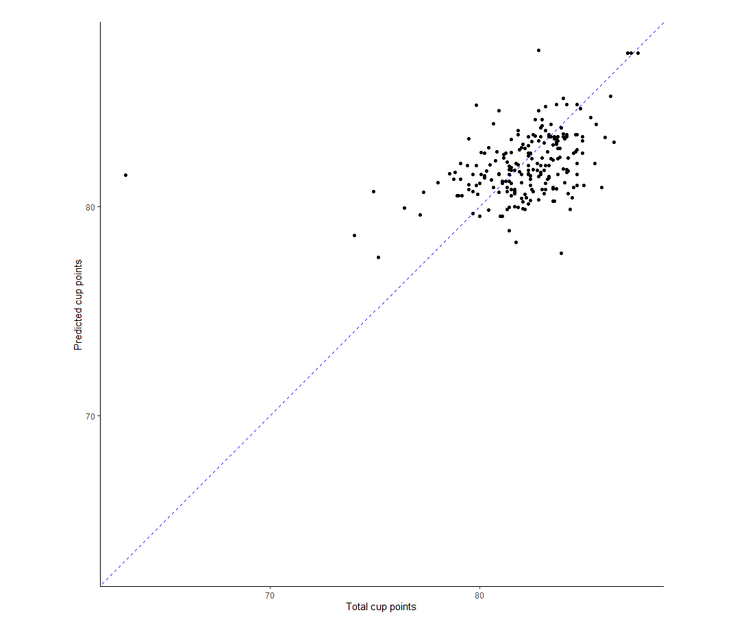
I find it most helpful to see it visually. So let’s just plot the predicted value vs true value using ggplot2. The chart is as below. On the whole, the model seems to do okay, but not great. In particular, there’s this really obvious outlier for which the actual score was below 70 but the model predicted >80. That’s very bad when you consider that most of the data seems to be clustered around the 80-85 points range.

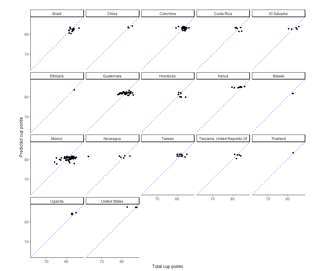
I think faceting by country shows quite clearly that the model has some way to go because there is a lot of horizontal spread present (e.g. Guatemala, Mexico), which suggests the model is missing out on some predictive power. Otherwise, we would expect to see broadly diagonal spread of the data (i.e. predicted value and true value broadly in line). In my defense, I think the data set is a bit light on predictors.

… and that’s it. That’s the basics of how to get started using tidymodel to build your own model.