Webscraping BTO application rates in R
Update (Mar 2022)
HDB seems to have updated their website such that the historical application rates are only available from Nov 2020. I also seem to have some issues with scraping Feb 2021 application rates which I have frankly not bothered to fix. Hence, the code which I used will need some updates to work properly. The csv file with my scraped data as of Sep 2020 can be found here.
Finally, for the curious reader, I ended up buying a resale property.
Original post as written in Sep 2020
(With some editorial edits)
Some context for any non-Singaporean readers who chance upon this - a Build-to-Order (BTO) flat is a public housing option that many Singaporean couples purchase as their first home. Typically, you would book a unit which will be completed only a few years later. BTO flats are (usually) released every quarterly. There’s just one twist: Those who want to purchase a BTO have to enter a ballot for a unit, and given that demand usually exceeds supply, there’s some serious luck* element involved here…
(* Despite the priority schemes available, anecdotally there’s a lot of luck involved.)
I haven’t had much luck in getting a good BTO queue number. The nature of a ballot means that maybe I’m just unlucky, but there is also a sense that there is a BTO undersupply. Is there publicly available data that we can use to check this? Well, kind of.
For those who have been through the process, you would be aware of the application status page on HDB’s website. It provides, for each BTO project-flat type, the number of units, applicants, as well as the respective application rates. In particular, I think the application rates serve as a rough measure of excess demand. So, if we can compare the application rates over time, then we can get a sense of how excess demand has evolved over time. Helpfully, although HDB only puts up the links for the three most recent BTO ballot, a quick check of the URL structure allow us to look up past ballot information (up to a point).
In turn, that means that we can use web scraping from all these different pages to put together a dataset for analysis, which I will go through here.
To simplify things a little, I’ll narrow the scope to what I’m really interested in:
- I will be focusing on the first-timer application rate for the rest of this post, because I am a first-timer myself, and I am most concerned with the first-timer application rate (basically my “competitors” in the ballot). Anecdotally, it seems that many of the people around me prefer to secure a flat before tying the knot officially, which may then have further implications down the line (e.g. when to have children). It may be worth noting that the definition of first-time application rate differs slightly for mature vs non-mature estates, though I’m not sure that it makes a substantive difference.
- I will also be focusing on 4-room or 5-room flats (henceforth referred to as “4R” or “5R”), which are my preferred flat types.
At a high-level, this is what we’ll be doing: The idea is to leverage on patterns in both the URL structure and the content layout in the respective pages to scrape data. Having done that, we would then need to apply some cleaning, possibly with some cross-checks, before producing visualisations in ggplot2. The libraries used are tidyverse, rvest, and lubridate.
One final note - this is my first time webscraping so I may not have implemented it as well as possible, but I think it also shows that this isn’t as hard as it seems.
Webscraping to build the dataset
Let’s go through the key parts of the webscraping approach.
We first need to identify the patterns in the URL structure. The first observation is that the URL structure is different for the latest launch (Aug 2020 at the point of writing) compared to previous launches. For Aug 2020, the URL is https://services2.hdb.gov.sg/webapp/BP13BTOENQWeb/AR_Aug2020_BTO?strSystem=BTO, but the ones for Feb 2020 and Nov 2019 are https://services2.hdb.gov.sg/webapp/BP13BTOENQWeb/BP13J011BTOFeb20.jsp and https://services2.hdb.gov.sg/webapp/BP13BTOENQWeb/BP13J011BTONov19.jsp respectively. So a reasonable guess is that we could amend the URL for Feb 2020/Nov 2019 and replace it with a previous month in which there was a BTO ballot to access the earlier BTO application information. That does turn out to be the case! For example, if we replace the Feb20 in the URL for Feb 2020 with Feb16 we can access the Feb 2016 info. Knowing the URL pattern means that we can feed the source URLs in easily later on.
period <- "Feb20" #define some period here, but let me just use Feb 2020 as an example

  if(period != "Aug20") {

    base_url <- "https://services2.hdb.gov.sg/webapp/BP13BTOENQWeb/BP13J011BTO"
    url <- paste0(base_url, period, ".jsp")

    } else if(period == "Aug20") {

      url <- "https://services2.hdb.gov.sg/webapp/BP13BTOENQWeb/AR_Aug2020_BTO?strSystem=BTO"
  }
Next, we need to identify where in each page we can obtain the information from. At a glance, the webpage looks reasonably static (a more dynamic website might present complications), and if we view the page source (right click -> view page source), we can see that the information does appear within the HTML code. This means that if we can identify patterns in the HTML code which isolate the information we want, then we can scrape that information without also bringing in things that we don’t want. In this case, it looked to me like the information was sitting within the <table class = "scrolltable"> tag, and that’s what I rely on to identify the relevant part of the HTML code.
 raw <- read_html(url)

 raw_tables <- html_nodes(raw, css = ".scrolltable") %>%
    html_table(trim = TRUE, fill = TRUE)

 table_2 <- raw_tables[[2]]
Believe it or not, at this point most of the webscraping is done. The code segments above provide the structure for scraping from one page. Because the BTO application rates are split across two tables (with one table for 2-room flexi flats), the code would bring in both tables. That’s not my interest here, so I use table_2 <- raw_tables[[2]] to take only the second table which contains info on 3R and above. The rest of the work lies in cleaning the raw data that has been scraped, and thinking about where there needs to be different treatment in either scraping or cleaning the data when extending this to cover the other pages.
Here’s what the Feb 2020 data looks like at this point. The scraping worked and what we want is largely there - compare against the original here - but at the same time, the two-tiered headers in the original page got imported in oddly, and the headers for the non-mature estate and mature estate categories got read in as a row on its own too, so there’s still some cleaning to do.
| Project | Flat Type | No of Units | Number ofApplicants | Application Rate^ | Application Rate^ | Application Rate^ | |
|---|---|---|---|---|---|---|---|
| 1 | Project | Flat Type | No of Units | Number ofApplicants | Non-Elderly | Non-Elderly | Non-Elderly |
| 2 | Project | Flat Type | No of Units | Number ofApplicants | First Timers | Second Timers | Overall |
| 3 | Non-Mature Town/ Estate | Non-Mature Town/ Estate | Non-Mature Town/ Estate | Non-Mature Town/ Estate | Non-Mature Town/ Estate | Non-Mature Town/ Estate | Non-Mature Town/ Estate |
| 4 | Sembawang (Canberra Vista) | 3-room | 124 | 847 | 3.7 | 14.1 | 6.8 |
| 5 | Sembawang (Canberra Vista) | 4-room | 385 | 3048 | 6.8 | 14.4 | 7.9 |
| 6 | Sembawang (Canberra Vista) | 5-room/ 3GEN | 266 | 3738 | 10.6 | 33.9 | 14.1 |
| 7 | Mature Town/ Estate | Mature Town/ Estate | Mature Town/ Estate | Mature Town/ Estate | Mature Town/ Estate | Mature Town/ Estate | Mature Town/ Estate |
| 8 | Toa Payoh (Toa Payoh Ridge) | 3-room | 102 | 935 | 4.3 | 103.8 | 9.2 |
| 9 | Toa Payoh (Kim Keat Ripples / Toa Payoh Ridge) | 4-room | 1211 | 11684 | 7.6 | 48.7 | 9.6 |
| 10 | TOTAL | TOTAL | 2088 | 20252 | 7.5 | 30.8 | 9.7 |
We want to fix the column headers and remove the headers/table dividers that got read in as rows. From our own contextual knowledge, we also know that the split between mature and non-mature estates is an important one for BTO application rates, so let’s try to preserve that info in a new variable.
#fix column names
    colnames(table_2) <- c("proj_name", "flat_type", "num_units", "num_applicants",
                       "first_timer_ratio", "second_timer_ratio", "overall_ratio")

mature_marker <- which(str_detect(table_2$proj_name, "Mature Town") &
                         !str_detect(table_2$proj_name, "Non-Mature Town"))


table_2 <- table_2 %>%
  mutate(date = period,
         temp_index = row_number(),
         estate_type = ifelse(temp_index >= mature_marker, "Mature", "Non-mature")) %>%
         #compare the row number against the mature marker and assign accordingly

 filter(str_detect(proj_name, "Project|Mature Town") == FALSE) %>%
 #remove the headers/dividers that got treated as entries

 mutate(proj_name = ifelse(proj_name == "TOTAL", paste("total",period, sep = "_"), proj_name)) %>%
 select(-temp_index)
The mature_marker tells us which is the row that contains the header for the mature estate. If we have correctly identified that, then given the structure of the table, we know that anything above (below) that is a project in a non-mature estate (mature estate). The last mutate is to preserve the total number of units which was scraped from the original. Strictly speaking, this is also something that we do not need as we can construct a total ourselves, but if we keep that information, we would be able to check for possible errors in the scraping/cleaning by comparing a constructed total against the scraped total. Here I modify the name to make it easy to identify which ballot period the total was for.
The data looks much better now (below). There’s probably more that can be done in terms of cleaning but maybe that can wait till later.
| proj_name | flat_type | num_units | num_applicants | first_timer_ratio | second_timer_ratio | overall_ratio | date | estate_type | |
|---|---|---|---|---|---|---|---|---|---|
| 1 | Sembawang (Canberra Vista) | 3-room | 124 | 847 | 3.7 | 14.1 | 6.8 | Feb-20 | Non-mature |
| 2 | Sembawang (Canberra Vista) | 4-room | 385 | 3048 | 6.8 | 14.4 | 7.9 | Feb-20 | Non-mature |
| 3 | Sembawang (Canberra Vista) | 5-room/ 3GEN | 266 | 3738 | 10.6 | 33.9 | 14.1 | Feb-20 | Non-mature |
| 4 | Toa Payoh (Toa Payoh Ridge) | 3-room | 102 | 935 | 4.3 | 103.8 | 9.2 | Feb-20 | Mature |
| 5 | Toa Payoh (Kim Keat Ripples / Toa Payoh Ridge) | 4-room | 1211 | 11684 | 7.6 | 48.7 | 9.6 | Feb-20 | Mature |
| 6 | total_Feb20 | TOTAL | 2088 | 20252 | 7.5 | 30.8 | 9.7 | Feb-20 | Mature |
The next step would be to wrap up these earlier steps in a function, and use map() to apply our defined function over a list of periods with available info.
get_bto_app_ratios_3Rplus <- function(period){

  if(period != "Aug20"){
    base_url <- "https://services2.hdb.gov.sg/webapp/BP13BTOENQWeb/BP13J011BTO"
    url <- paste0(base_url, period, ".jsp")
    } else if(period == "Aug20") {
      url <- "https://services2.hdb.gov.sg/webapp/BP13BTOENQWeb/AR_Aug2020_BTO?strSystem=BTO"
  }

  raw <- read_html(url)

  raw_tables <- html_nodes(raw, css = ".scrolltable") %>%
    html_table(trim = TRUE, fill = TRUE)

  table_2 <- raw_tables[[2]]

  colnames(table_2) <- c("proj_name", "flat_type", "num_units", "num_applicants",
                       "first_timer_ratio", "second_timer_ratio", "overall_ratio")


  mature_marker <- which(str_detect(table_2$proj_name, "Mature Town") &
                         !str_detect(table_2$proj_name, "Non-Mature Town"))

  table_2 <- table_2 %>%
  mutate(date = period,
         temp_index = row_number(),
         estate_type = ifelse(temp_index >= mature_marker, "Mature", "Non-mature")) %>%
         #compare the row number against the mature marker and assign accordingly

 filter(str_detect(proj_name, "Project|Mature Town") == FALSE) %>%
 #remove the headers/dividers that got treated as entries

 mutate(proj_name = ifelse(proj_name == "TOTAL", paste("total",period, sep = "_"), proj_name)) %>%
 select(-temp_index)


  print(paste("Scraped", period))
  return(table_2)
}
Before using map() though, we need to look across the other HDB pages for oddities that may significantly affect the scraping. For instance, one notable issue is that prior to Nov 2015, the application rates were displayed as only one table, rather than two, which means that for those periods, we would have to modify table_2 <- raw_tables[[2]] to table_2 <- raw_tables[[1]]. These older tables also have an additional column for singles application rate, which is no longer present in the newer ones. There are also some differences and inconsistencies in the table headers over time. Most of these differences I spotted while manually browsing - perhaps there’s a more technically elegant way to check for such things, but unfortunately I don’t know them at this time.
The modifications to the steps in the function turn out to be a bit fiddly, so I’ll skip the detailed explanation here. You can take a look at the full code here. (You can also make your life easier and deal with less modifications if you focus on a smaller time period.)
Finally, it’s worth noting at this point that the oldest available info I could find (following the URL structure set out earlier) was for Sep 2014. It could be that the info is simply not available online anymore, or is under a different URL structure - who knows? Regardless, that still gives us 5 complete calendar years of data. Not too shabby, I think.
Once we’re done modifying and defining the function, let’s bring the data in. I also create a csv just to preserve a raw copy of the data as-scraped, which I find this helpful for pinpointing where things have gone wrong if there are subsequent problems, but of course it’s not strictly necessary.
  all_periods <- c("Aug20", "Feb20",
                   "Nov19", "Sep19", "May19", "Feb19",
                   "Nov18", "Aug18", "May18", "Feb18",
                   "Nov17", "Aug17", "May17", "Feb17",
                   "Nov16", "Aug16", "May16", "Feb16",
                   "Nov15", "May15", "Feb15",
                   "Nov14", "Sep14")

  combined_data <- map_df(all_periods, get_bto_app_ratios_3Rplus)

  write_csv(combined_data, "scraped_data.csv")

  str(combined_data)
tibble [253 x 9] (S3: spec_tbl_df/tbl_df/tbl/data.frame)
 $ proj_name         : chr [1:253] "Choa Chu Kang (Keat Hong Verge *)" "Choa Chu Kang (Keat Hong Verge *)" "Tengah (Parc Residences @ Tengah)" "Tengah (Parc Residences @ Tengah)" ...
 $ flat_type         : chr [1:253] "3-room" "4-room" "3-room" "4-room" ...
 $ num_units         : num [1:253] 118 290 99 281 184 144 706 438 240 140 ...
 $ num_applicants    : num [1:253] 263 683 363 1436 1284 ...
 $ first_timer_ratio : chr [1:253] "1.5" "2.1" "2.5" "4.3" ...
 $ second_timer_ratio: chr [1:253] "4.1" "8.4" "6.5" "9.6" ...
 $ overall_ratio     : num [1:253] 2.2 2.4 3.7 5.1 7 6.2 5.8 9.8 10.7 21.5 ...
 $ date              : chr [1:253] "Aug20" "Aug20" "Aug20" "Aug20" ...
 $ estate_type       : chr [1:253] "Non-mature" "Non-mature" "Non-mature" "Non-mature" ...
 - attr(*, "spec")=
  .. cols(
  ..   proj_name = col_character(),
  ..   flat_type = col_character(),
  ..   num_units = col_double(),
  ..   num_applicants = col_double(),
  ..   first_timer_ratio = col_character(),
  ..   second_timer_ratio = col_character(),
  ..   overall_ratio = col_double(),
  ..   date = col_character(),
  ..   estate_type = col_character()
  .. )
There’s clearly some cleaning to be done here. The first timer ratio - a key variable of interest - is a character, not numeric. It’s probably also useful to create a proper date variable for use later. I do some cleaning below to create proper date variables, clean out the flat types a bit, and address some type issues. There are warning messages when forcing the application rates to numeric but it’s not a big deal in this case - it’s because some of the application rates for older studio apartment releases have “NA” or “Not applicable” entries. Those are not the focus here so we can just move on.
clean_combined <- combined_data %>%

  #create a proper date variable
  separate(date, into = c("month", "year"), sep = 3) %>%
  mutate(year = as.numeric(year),
         year = as.character(2000 + year),
         date = paste("01", month, year, sep = "-")
         ) %>%

  #clean flat type categories
  mutate(flat_type = ifelse(flat_type == "", "TOTAL", flat_type),
         flat_type = if_else(str_detect(flat_type, "5-room"), "5-room", flat_type)) %>%
          #some 5-rooms was also tagged as 3GEN. I've simplified them to all be treated as 5-room flats

  #deal with variable types (e.g. parse date)
  mutate(date = dmy(date),
         year = year(date),
         estate_type = as.factor(estate_type)) %>%

  mutate(across(matches("num|ratio"),as.numeric))
The data is a bit cleaner now, and we should do a cross-check to catch any errors in the webscraping. As I mentioned earlier, one way to cross-check that is to compare constructed totals of the scraped info, against the totals that were scraped from the web. We can do that by temporarily filtering out the scraped totals and then re-joining the constructed total with the cleaned data, then compare the two totals. stopifnot() will throw up an error if the two totals are not identical. When we’re satisfied with the cross-check, we can throw out the scraped totals as we can produce construct totals if those are necessary.
By the way, I recall using the assertive package in the past but I seem to have had some problems with it recently, which is why I went with stopifnot().
  crosscheck1 <- clean_combined %>%

    #construct a total from all non-total entries
    filter(str_detect(proj_name, "total_") == FALSE) %>%
    group_by(date) %>%
    summarize(num_units  = sum(num_units)) %>%


    #after joining, I should now have both the scraped totals and the constructed totals
    full_join(clean_combined, by = "date") %>%
    filter(str_detect(proj_name, "total_"))


  #if not identical, something has gone wrong and we should check for errors
  stopifnot(identical(crosscheck1$num_units.x, crosscheck1$num_units.y))

  #throw out scraped totals
  clean_combined <- clean_combined %>%
    filter(str_detect(proj_name, "total_") == FALSE)
And now we’re ready for some plots!
Some exploratory plots
Nothing too fancy here, just some basic plots to build our understanding of the excess demand. Let’s look at the supply side first - what does the supply of 4R and 5R flats look like?
  clean_combined %>%

    #filter out 2014 because incomplete year
    #filter only 4 or 5 rooms because that's the interest
    filter(year > 2014, str_detect(flat_type,"4-room|5-room")) %>%

    group_by(year, estate_type) %>%
    summarize(num_units  = sum(num_units)) %>%

    mutate(year_total = sum(num_units),
           plot_alpha = ifelse(year == 2020, 0.7, 1)) %>%
          #plot_alpha is a helper variable for making the 2020 bar translucent

    ggplot(aes(x = as.factor(year), y = num_units, fill = estate_type, alpha = plot_alpha)) +
      geom_col() +
      geom_text(
        aes(label = num_units),
        position = position_stack(vjust = 0.5)
      ) +

    scale_alpha_continuous(range = c(0.7,1), guide = "none") +

    labs(
      title = "Number of 4R/5R BTO flats (annual)",
      x = "",
      y = "",
      fill = ""
      ) +

    theme_classic() +
    theme(legend.position = "bottom")
which produces this:
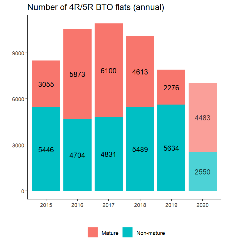
It looks like the total supply of 4R/5R BTO flats increased from 2015-2017, but have fallen since. The bars for 2020 are set to translucent to indicate that the number is not directly comparable because there is still the Nov 2020 ballot which is not part of this data yet. However, it does look very possible that after the Nov 2020 supply is in, the total for 2020 will surpass that of 2019. What is less clear is whether this is a sustained change or not.
What about the demand side? The steps to do this are very similar to the earlier lines for the supply, so I won’t repeat them here. Just replace all the num_units with num_applicants, change the plot title, and we’re set to go.
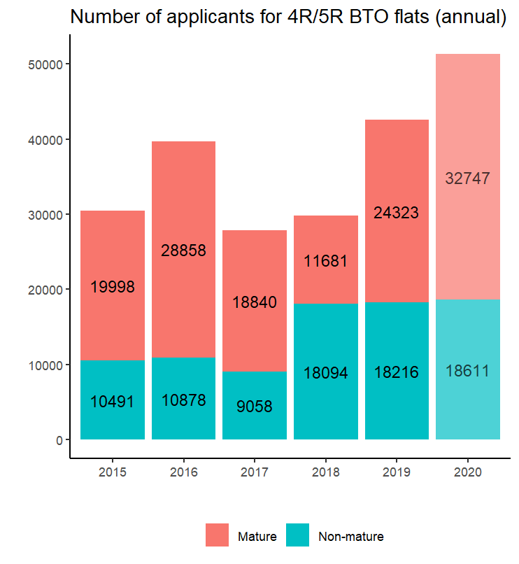
I’m not sure what happened in 2016, but aside from that possible anomaly, it’s a clear upward trend. In particular, the total applicants in 2020 have already exceeded the totals for 2019, even though there’s still the Nov 2020 ballot to go!
Some might argue that this increase is because of more speculative second-time buyers entering the ballot due to some BTO launches which are perceived to be exceptional launches, or because the longer estimated build times driven by COVID-19 or perception of better BTO launches are drawing more speculative applications from younger couples. For the first reason, the publicly available data doesn’t have enough granularity to allow us to separate out the second-timer applicants. For the latter two reasons, well, if they are first-timers too, then whatever the reason, the end result is still greater excess demand in the pool…
Regardless, I’d take this with a pinch of salt just purely because of the inability to separate out the second-timer applicants.
Finally, on to the main interest - the first-timer application rates.
  clean_combined %>%

    #filter out 2014 because incomplete year
    #filter only 4 or 5 rooms because that's the interest
    filter(year > 2014, str_detect(flat_type,"4-room|5-room")) %>%

    ggplot(aes(x = date, y = first_timer_ratio, color = estate_type)) +

      geom_point(alpha = 0.6, size = 3) +

      geom_hline(yintercept = 1, linetype = "dashed") +

      scale_x_date(date_breaks = "1 year", labels = year) +

      labs(
        title = "BTO first-timer application rate for 4R/5R (by project)",
        x = "",
        y = "",
        color = ""
      ) +

      theme_classic() +
      theme(legend.position = "bottom")
which produces this:
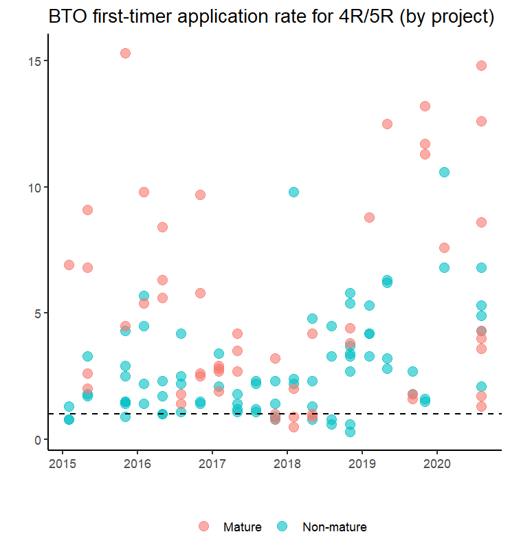
For reference, I have included a dashed line to indicate where the first-timer application rate = 1, so points above the dashed line indicate the presence of excess demand (and vice versa). To be clear, I am not saying that it is necessarily better from a policy perspective for the rate to be below 1 (i.e. no excess demand). But certainly from an applicant perspective, I would be happy to see lower application rates.
It actually looks a bit messy, but here’s what I see:
- Most launches since 2015 have first-timer application rates which exceeds one, so there’s almost always greater demand than supply. Prior to 2019, some launches actually had first-timer ratios below one, and it looks like most of them happened between late 2017 to end-2018.
- Quite a number of launches between 2015-2016 had first-timer application rates above five, but they were mostly mature estate launches so that might explain the popularity. Between 2017 and 2019, very few launches had a first-timer application rate above five. However, from 2018 onwards, we start seeing the higher applications rates return.
- To my eyes, it looks like the overall cluster of first-timer application rates have gone up since 2018. Quite a number of mature estates start seeing first-timer applicant rates beyond ten, and even the ratios for the non-mature estates look like they are edging up. Ten applicants competing for a unit! No wonder it’s so hard to get a good queue number.
- I think the trend in the ratios (high in 2015-2016, fell in 2017-2018, then increased again since), fits broadly with what we saw earlier about the number of units offered and applicants. We saw that the supply of 4R+ BTO flats increased from 2015-2017, then decrease since, and possibly looks to be increasing again this year (relative to 2019). So the dip in ratios in 2017-2018 may be because more applicants were “cleared” off the market in 2016-2017. As for demand, the number of applicants have really jumped in 2019 and 2020, so maybe that’s driving the ratios in 2019 and 2020. This is all a bit speculative of course, given that we don’t have more in-depth or granular data to study this.
In any case - let’s take a look at the same plot but separating the mature estates from the non-mature estates using facet_grid(). This time I also set the size of the point to reflect the number of units offered. (I didn’t do it previously because it would clutter the plot even further.)
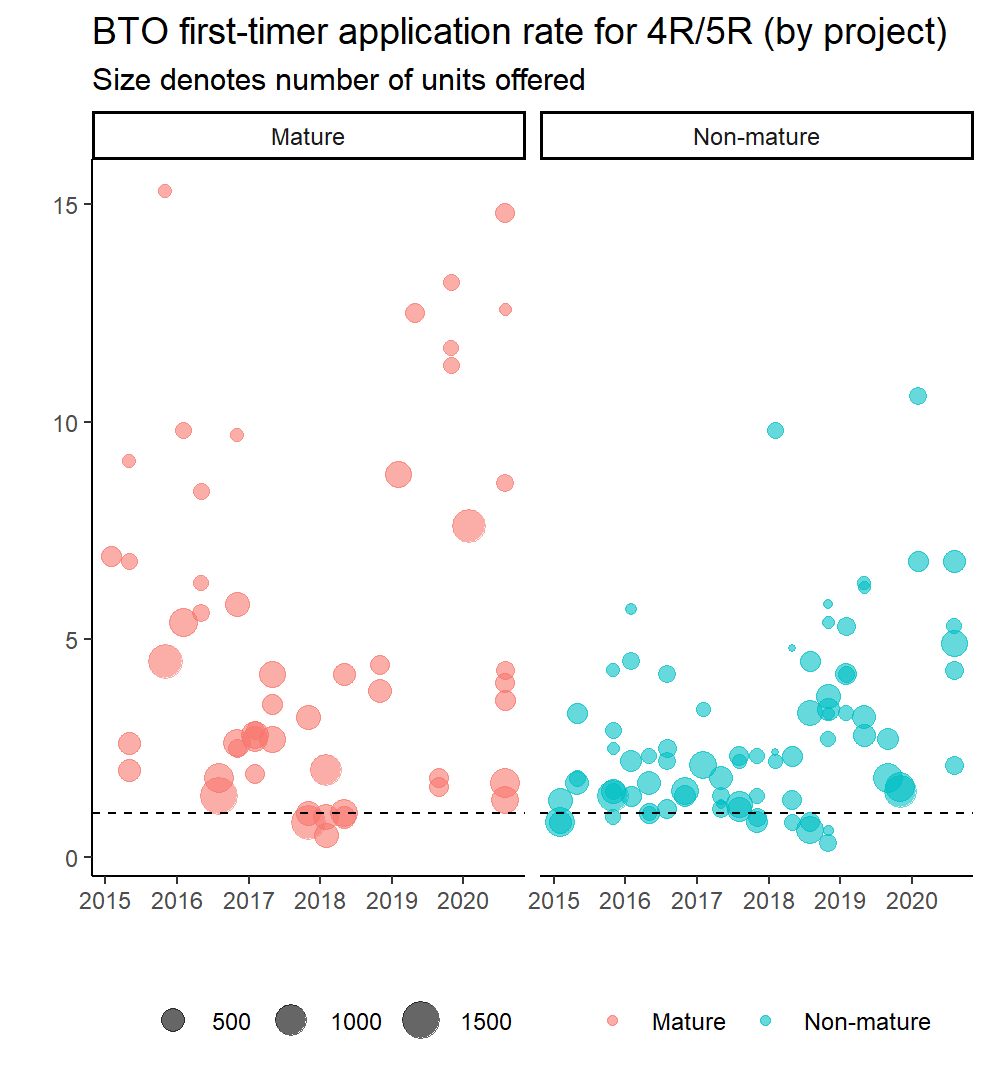
I don’t think this reveals anything particularly new. But I think the edging up in the first-timer application rates for the non-mature estates is more obvious here, and for the mature estates it does look to me like a U-shaped trend in the application rates.
Anyway, that’s it for now. Leaving aside whether you agree (or not) with my interpretation of the plots, I hope this has shown that webscraping is more accessible than you might have realised. For anyone interested, the full R script used, including the amended scraping function to account for differences in table structure over time, can be found here. If you are reading this when the next ballot has launched (currently scheduled for Nov 2020), it is likely that you’d have to amend the function to read in the new URL for Aug 2020 and include the URL for Nov 2020 to get the webscraping working properly.